
Down the Rabbit Hole with Perf
Published:
In my previous post, I described the implementation of two lock-free algorithms for recursive queries in graph databases that achieved speedup through atomic operations and parallel BFS traversals. In this post, I will share some interesting performance findings I encountered while optimizing both algorithms using Linux Perf.
Tuning code for performance is never straightforward. It requires an intricate understanding of what’s happening under the hood, knowing where to look, and knowing the right tool to use. Linux Perf is a powerful tool for this job - it provides rich metrics about CPU cycles, cache misses, TLB misses, branch predictions, and more. If you’re looking for a deeper dive on Perf, I recommend this tutorial.
This post is divided into four sections. The first section briefly describes the algorithms we will tune for performance, and the scheduling policy that runs them in Kùzu (more details in the VLDB ‘25 paper). The next two sections describe interesting performance findings: Section 2 describes how a parameter introduced too much concurrency leading to performance degradation and Section 3 describes how Perf revealed a performance bottleneck and how prefetching helps tackle it. The final section, similar to the previous post, discusses certain hardware requirements for performing such low-level optimizations.
Table of Contents
Background
In this section, I will briefly describe the hybrid scheduling policy we implement in Kùzu to parallelize recursive queries and the variable length recursive query returning paths that I will optimize for performance in this post.
nTkS Scheduling Policy
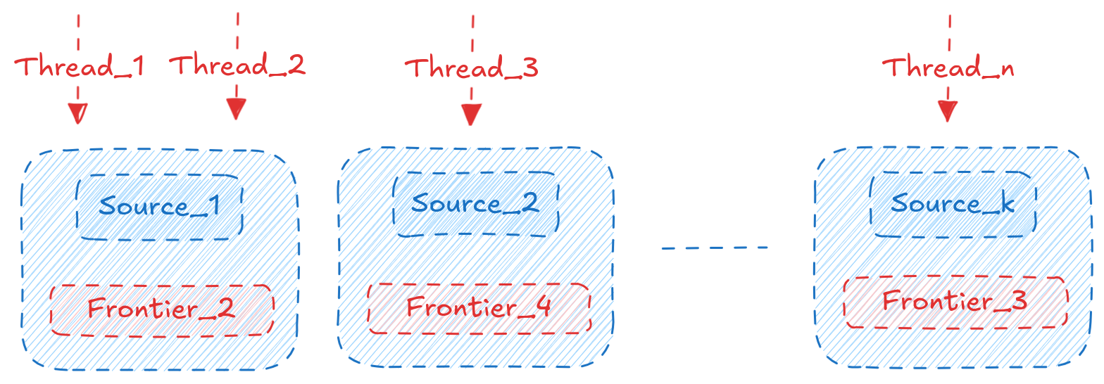
The nTkS scheduling policy is a hybrid policy that combines vanilla morsel-driven parallelism implemented in analytical databases with frontier parallelism (parallel BFS) implemented in graph analytics systems such as Ligra and Pregel. Where morsel-driven parallelism assigns Threads to execute on a partition of input tuples (table rows or index entries or intermediate results), frontier parallelism assigns Threads to execute on a partition of the graph frontier (vertices). We combine both these approaches to achieve better performance. The n in nTkS refers to the number of Threads running concurrently and k refers to the number of sources whose recursive computation is being performed on. As an example, consider the following query:
MATCH p = (a:Person)-[r:Knows* SHORTEST 1..30]->(b:Person)
WHERE a.ID > 10 AND a.ID < 21
RETURN length(p)
This query runs the shortest path algorithm starting from 10 source vertices (i.e., a.ID from 11 to 20). If we set n=4 and k=2, then at any point in time, 4 threads will be running concurrently, and exactly 2 sources will be active. The threads decide which source to execute on depending on the size of the frontier and how many threads are already executing on that source. More details about the scheduling policy are in the paper.
Variable Length Recursive Query
The variable length recursive query is expressed in Cypher as follows:
MATCH p = (a:Person)-[r:Knows* 1..5]->(b:Person)
WHERE a.ID = srcID AND b.ID = dstID
RETURN p
The above query returns all paths from a source vertex srcID to a destination vertex dstID with a length between 1 and 5. I’ve described the lock-free parallel implementation to execute this query in my previous post. The key thing to remember is that this algorithm is compute-intensive since it keeps track of all paths (including cycles) and is a good candidate for performance tuning.
The curious case of ‘k’
One of the core parameters in the nTkS policy is the number of sources, k, that we allow to run in parallel. Intuitively, increasing k should improve runtime — the more sources we process simultaneously, the better we utilize available cores and memory bandwidth.
An alternative and more simple scheduling policy would be to simply run a single source at a time, parallelizing it across all available threads. This way, we don’t need to worry about assigning threads across multiple sources. However, this approach leads to underutilization in practice since we are not able to parallelize a single source enough and get enough throughput. We tested varying k on the following real-world + synthetic datasets:
| |V| | |E| | Avg Degree | |
|---|---|---|---|
| LDBC-100 | 448,626 | 19,941,198 | 44 |
| LiveJournal | 4,847,571 | 68,993,773 | 14 |
| Spotify | 3,604,454 | 1,927,482,013 | 535 |
| Graph500-28 | 121,242,388 | 4,236,163,958 | 35 |
We ran a recursive join query, starting from 64 sources, keeping the total threads fixed at 32 while varying k from 1 to 32 to see its effect on runtime. The following figure shows the improvement factor in runtime compared to k=1 for each dataset:
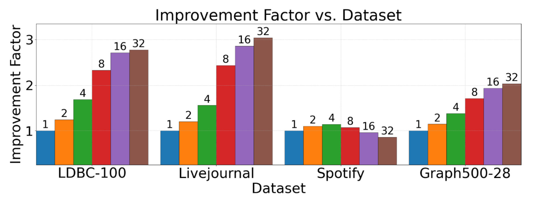
As we notice from the figure, for most graphs (LDBC, LiveJournal, Graph500), increasing k leads to better performance with speedups of 2-3x, but for Spotify, increasing k actually leads to worse performance! Compared to the other datasets, Spotify has a very high average degree (535) and this means that even a single source has a lot of parallelism to exploit. This is where Linux Perf helped us identify the issue. We used perf stat to collect metrics for our query:
| Dataset | Metric | k=1 | k=2 | k=4 | k=8 | k=16 | k=32 |
|---|---|---|---|---|---|---|---|
| LDBC-100 | Time (s) | 4.1 | 3.3 | 2.3 | 1.5 | 1.3 | 1.2 |
| LLC Tp | 10.9 | 11.4 | 13.9 | 19.4 | 23.6 | 23.9 | |
| LiveJournal | Time (s) | 37.5 | 31.2 | 22.6 | 13.5 | 10.3 | 9.7 |
| LLC Tp | 6.2 | 6.5 | 7.2 | 9.5 | 10.7 | 10.9 | |
| Spotify | Time (s) | 82.8 | 71.8 | 68.7 | 73.0 | 82.8 | 95.6 |
| LLC Tp | 40.4 | 48.5 | 50.1 | 48.6 | 43.1 | 38.2 | |
| Graph500-28 | Time (s) | 938.9 | 766.0 | 640.0 | 492.9 | 449.9 | 432.0 |
| LLC Tp | 12.7 | 15.1 | 17.2 | 21.2 | 23.0 | 24.0 |
This table is dense, so let’s unpack it step by step. We’re examining the relationship between runtime and LLC (last level cache) throughput. The LLC is the largest and slowest cache in the memory hierarchy, and it is shared among all cores. The ideal scenario is to have LLC loads / LLC throughput achieved increase, as we increase the parameter k. Better the LLC throughput, less time the CPU has to wait for data from main memory. Across 3 datasets (LDBC, LiveJournal, Graph500), we see that as k increases, the LLC throughput also increases, leading to better performance. However, for Spotify, we see LLC throughput slightly increase from k=1 to k=4, but then it starts decreasing. Another interesting observation is that the runtime for Spotify starts increasing from k=4 onwards as well. These metrics confirm two key observations:
- LLC throughput is a good proxy for performance in our workloads since we are memory bound, lower runtime always corresponds to higher LLC throughput from the table.
- Spotify even with
k=1achieves very high LLC throughput (40.4 Million/s) compared to the other datasets (6.2-12.7 Million/s), indicating it parallelizes well even with a single source. Increasingkbeyond 4 leads to too much concurrency and contention for memory bandwidth, leading to lower LLC throughput and higher runtime.
The underlying cause becomes clear when we visualize cache access patterns. Figure c shows how threads access cache when processing sparse graphs (LDBC, LiveJournal, Graph500), while Figure d shows the pattern for Spotify’s dense graph.
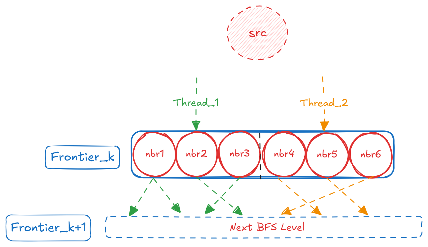
In sparse graphs, threads exhibit minimal cache overlap when processing a single source, limiting parallelization effectiveness. Additional concurrent sources (k > 1) provide independent work that better utilizes available cache capacity and memory bandwidth.
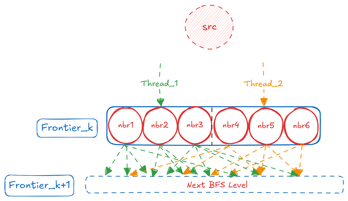
Spotify’s high average degree (535) creates substantial cache overlap even with a single source—threads naturally access related data, achieving 50 Million LLC loads/s at k=4. Beyond this point, additional sources create interference and bandwidth contention rather than productive parallelism. Overall, this was an interesting use case of Perf helping us identify a performance anomaly and understand how increasing / decreasing concurrency at the software level affects the underlying hardware. In the next section, I will describe another interesting use case of Perf helping us identify a performance bottleneck and certain tricks to tackle it.
The Art of Prefetching
Imagine calling a restaurant to place your order before you leave home. By the time you arrive, your food is already prepared. Why waste time waiting when you could have started the process earlier? Of course, this only works if you time it right — call too early and your food gets cold while you’re stuck in traffic. Call a restaurant that’s already slammed, and the kitchen won’t get to your order any faster anyway. But when conditions are right, this simple idea—requesting something before you need it—is how CPU prefetching works. In this section, we will try and experiment with applying software prefetching to an expensive query - the variable length recursive query returning paths:
    MATCH (a:lj_node)-[r:lj_rel* 1..5]->(b:lj_node)
    WHERE a.id < $id1 AND b.id < $id2
    RETURN r;
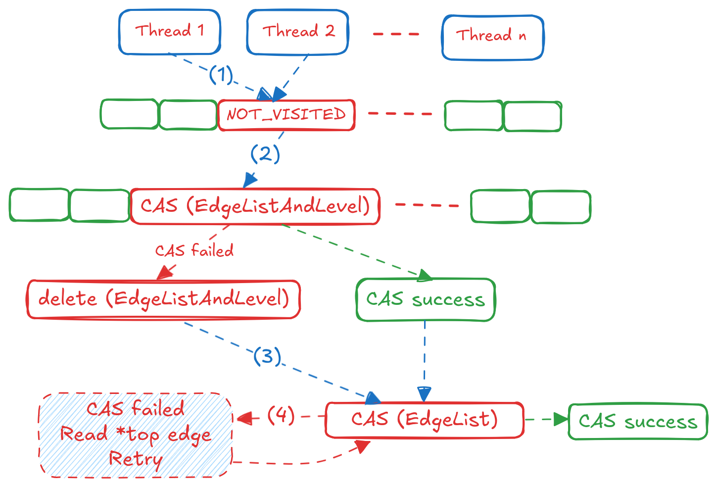
I’ll skip the details of the algorithm since I’ve described it in my previous post. To recap, the high level flow of how the algorithm works is as follows:
When we run this query on the LiveJournal dataset, for a sample query with 50 sources, 500 destinations and upper bound of 5, we get a runtime of ~27 seconds with a result of 138,471 paths. Let’s start to dig in and understand where CPU cycles get spent for this query using perf record and tracking the cycles event:
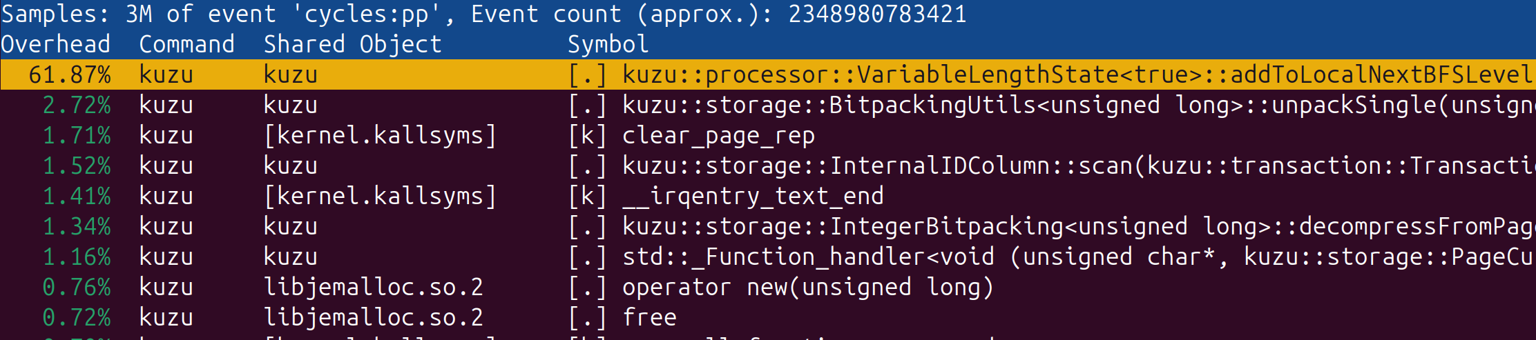
(Unsurprisingly) the top function where CPU cycles are spent is the var-len function which adds new neighbours encountered to the next frontier. When we dig deeper into this function, to find out which lines are the most expensive, we find the following:
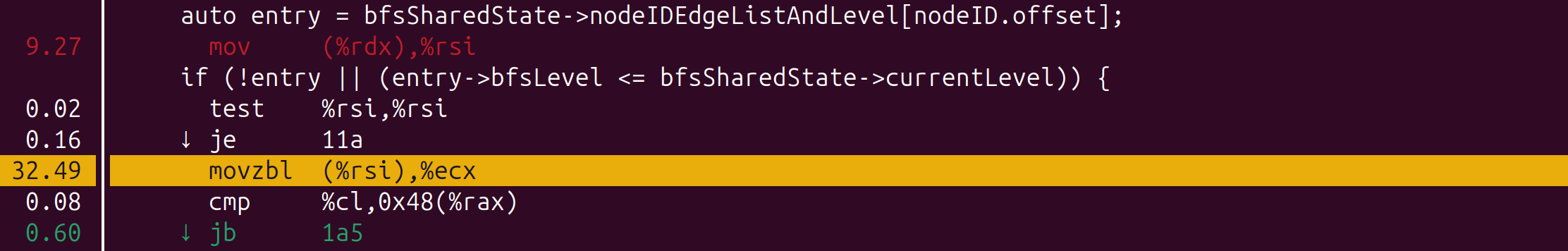
From Figure e’s flow chart, this line corresponds to Step (2), where a Thread reads the EdgeListAndLevel information of a neighbour, to confirm if it was already encountered at this BFS level or not.
auto entry = bfsSharedState->nodeIDEdgeListAndLevel[nodeID.offset];
mov     (%rdx), %rsi
if (!entry || (entry->bfsLevel <= bfsSharedState->currentLevel)) {
  test    %rsi, %rsi
  je      11a
  movzbl  (%rsi), %ecx          # ← 32.49%
  cmp     %cl, 0x48(%rax)
  jb      1a5
}
The movzbl is a load instruction, in this case it is taking the address (saved in rsi register), dereferencing it and placing the object in the ecx register. This instruction costs the most because it is causing CPU stalls from the CPU having to wait for the data to be fetched from memory to the cache, in this case the bfsLevel variable of the EdgeListAndLevel struct. In other words, we are again memory bound, we are unable to feed the CPU fast enough. This is where software prefetching comes in:
- We will use a two stage prefetching mechanism, we will first prefetch the pointer to the structs itself ahead of the elements and then once we are sure that the pointer is in the cache, we will prefetch the
bfsLevelvariable. - We will try to prefetch not just the
bfsLevelvalue, but also any other variable we are sure we are going to read soon (such as the visited state -Step (1)in Figure e)
With these two changes, the brief pseudocode would look something like this:
visited_nbrs(nbr_node, nbr_offset, edge_offset, src_node_level) {

    // Stage 1: Prefetch entry pointer
    if (nbr_offset + 2 * PREFETCH_DISTANCE) {
        auto future_pos = nbr_offset + 2 * PREFETCH_DISTANCE;
        auto future_node = nbr_nodes[future_pos];
        __builtin_prefetch(NodeEdgeListAndLevels[future_node], 0, 0);
    }

    // Stage 2: Prefetch the actual fields
    if (i + PREFETCH_DISTANCE < totalEdgeListSize) {
        auto future_pos = nbr_offset + PREFETCH_DISTANCE;
        auto future_node = nbr_nodes[future_pos];
        if (auto future_entry = NodeEdgeListAndLevels[future_node]) {
            // Prefetch the first cache line, contains bfsLevel
            __builtin_prefetch(future_entry, 0, 0);
        }
        // Prefetch the global visited status as well
        __builtin_prefetch(global_visited[future_node], 0, 0)
    }

   ....
   // same steps as before from 1-4 in Figure (e)
   ....
}
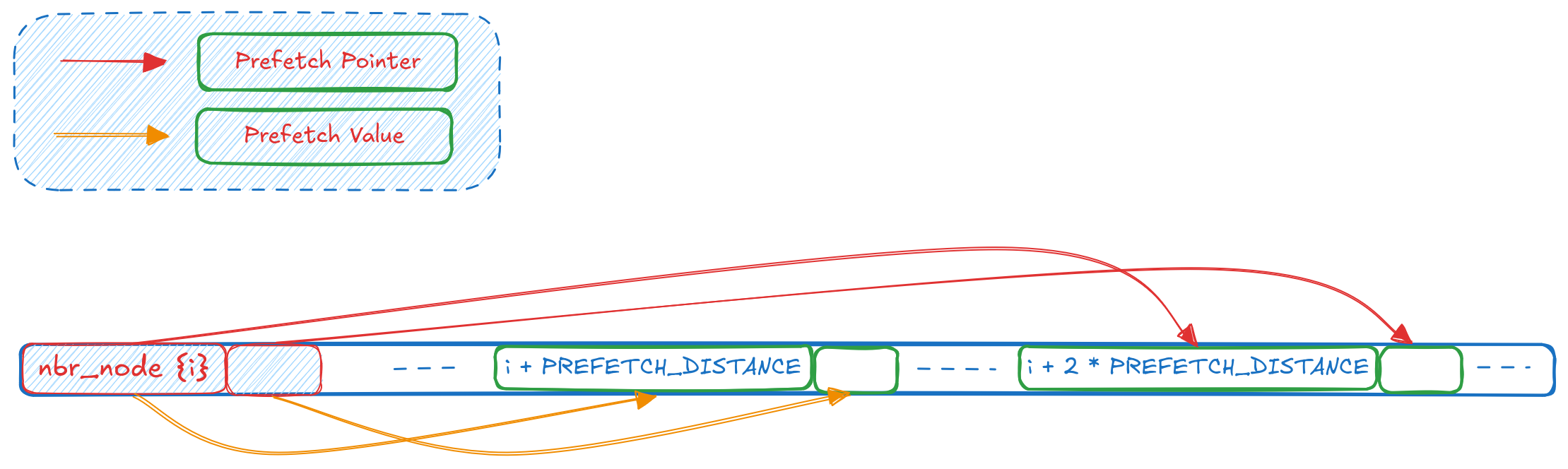
The PREFETCH_DISTANCE is a heuristic chosen which decides from what distance of the current neighbour position, do we want to prefetch values. This value would depend on the approximate latency of fetching data from memory and, total CPU cycles for one iteration of the loop to execute. If we were to visualize the positions that we are prefetching, the following figure highlights this:
With this, our prefetch logic is in place. A rerun of the same query now takes ~20 seconds to run, which is about ~26% improvement. If we look at the perf record trace of the cycles event again, and we see:
auto entry = bfsSharedState->nodeIDEdgeListAndLevel[nodeID.offset];
mov     (%rdx), %rsi
if (!entry || (entry->bfsLevel <= bfsSharedState->currentLevel)) {
  test    %rsi, %rsi
  je      182
  movzbl  (%rsi), %ecx          # ← 6.63%
  cmp     %cl, 0x48(%rax)
  jb      1a5
}
The % of CPU cycles on the movzbl instruction has been reduced to ~6.6% where it was ~32.5% before. While there was an overall improvement in runtime (26%), the heuristics and complexity of implementation sort of outweigh the benefits, unless the query is really sensitive to latency maybe ?
So, what’s the catch?
As we saw in both sections, Linux Perf proved invaluable for identifying performance hotspots in our algorithms, but relying on this level of profiling is not always feasible. The insights gained from profiling on specific hardware can easily become obsolete when moving to systems with completely different microarchitectures. For example, the optimal parameter k we determined for our graphs in Section 2 would likely change on a machine with a larger LLC (L3) cache. On such hardware, even higher values of k for Spotify might yield better performance, since a larger cache typically comes with higher memory bandwidth.
Another important consideration is that our queries had a clearly identifiable bottleneck from the start—the recursive computation was the single performance hotspot we needed to optimize. In real-world workloads, however, performance bottlenecks tend to be distributed across multiple operations, and there is rarely a single silver bullet that delivers substantial gains.
Finally, there is the question of marginal gains. We invested significant effort to identify that we were memory-bound and implemented prefetching to address it. First, getting prefetching right is extremely difficult and requires significant experimental iteration. The PREFETCH_DISTANCE is entirely heuristics-based and demands manual tuning for each system. What I didn’t mention in Section 3 is that my initial prefetch implementation actually degraded performance—I mistakenly prefetched too aggressively in a loop instead of selectively prefetching specific pointers or values ahead of time. While I eventually achieved measurable improvements, the experience highlights a fundamental challenge in low-level performance engineering: diminishing returns. The deeper you optimize, the smaller the gains relative to the effort invested.