
Anatomy of a Lock-Free Algorithm
Published:
In this post, I’ll describe parallel implementation of two graph algorithms: (i) shortest path (ii) variable length recursive join that returns full paths – both implemented using atomic (lock-free) primitives for high performance. This is the first of two posts and is meant to be a companion to my VLDB ‘25 paper. The paper focuses more on runtime scheduling policies whereas this post will specifically delve into how we parallelize these operators.
| Shortest Path | Variable Length | |
|---|---|---|
| 1 thread | 1890 ms | 416 sec |
| 32 threads | 274 ms (7x) | 27 sec (16x) |
The blog is divided into four sections. The first section provides a quick primer on recursive join queries, while the next two sections describe parallel algorithms for shortest path and variable-length queries. These two algorithms sit at opposite ends of the spectrum: the (unweighted) shortest path query, which returns only path lengths, is relatively straightforward in terms of what needs to be tracked and how to parallelize it. In contrast, the variable-length path query, which returns full paths, is among the most expensive queries a graph database can execute, both in terms of computation and memory. Finally, I discuss the challenges encountered while running these queries and highlight how beneficial lock-free algorithms really are in practice.
Table of Contents
Background
It’s 2025, and most graph databases now support Cypher as a query language (finally some consolidation here). Expressing many-to-many joins (long join patterns) or recursive queries in Cypher is way more intuitive than in SQL. When I say “recursive queries” here, I mean queries that repeatedly expand joins until a condition is satisfied. The condition can be for example, encountering a particular node (shortest path) or reaching a particular join depth (variable length). In Cypher, if you wanted to write the unweighted shortest path query, and return the path length, this would be the syntax:
MATCH p = (a:Person)-[r:Knows* SHORTEST 1..30]->(b:Person)
WHERE a.name = 'Alice' AND b.name = 'Bob'
RETURN length(p)
The above query would take the node ‘Alice’, explore who Alice knows (1 join) then explore their neighbours (2 joins) and keep going until we hit ‘Bob’. We “recursively” keep exploring until we either hit our destination or we hit the upper bound (specified after the SHORTEST keyword). Now compare this to a variable length recursive join query:
MATCH p = (a:Person)-[r:Knows* 1..10]->(b:Person)
WHERE a.name = 'Alice' AND b.name = 'Bob'
RETURN p
This query is a bit different, as it does not have the SHORTEST keyword, it will compute all paths of up to length 10 that end at ‘Bob’. This is an example of the variable length (var-len) recursive join. There are different semantics for running the var-len recursive query, and depending on the semantics the query engine may have to keep track of cycles. For the scope of this blog, we will focus on the SIMPLE path semantics, that allows repeating both nodes and edges in the path. Let’s make this more concrete with an example graph:
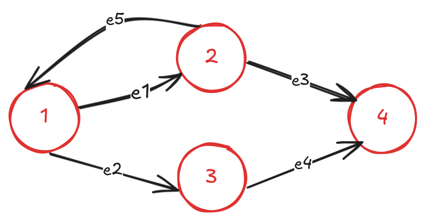
If a user ran the SHORTEST path query from node (1) to node (4), the result would return the path: (1)-[e1]->(2)-[e3]->(4). If we need all the shortest paths, we could specify ALL SHORTEST in our query and get back (1)-[e2]->(3)-[e4]->(4) as well. Now if we ran the var-len recursive query between (1) and (4), with SIMPLE path semantic, the paths returned would be (1)-[e1]->(2)-[e3]->(4), (1)-[e1]->(2)-[e5]->(1)-[e1]->(2)-[e3]->(4) and so on until the upper bound of the query is reached. Since there is a cycle in the graph, the query engine would have to keep track of the cycles unlike the shortest path query that visits every node only once.
Now that we have the background about different recursive joins, let’s look at the implementation of the parallel lock-free algorithms.
Shortest Path
The Cypher query we’re trying to parallelize here is:
MATCH p = (a:Person)-[r:Knows* SHORTEST 1..30]->(b:Person)
WHERE a.name = 'Alice'
RETURN length(p)
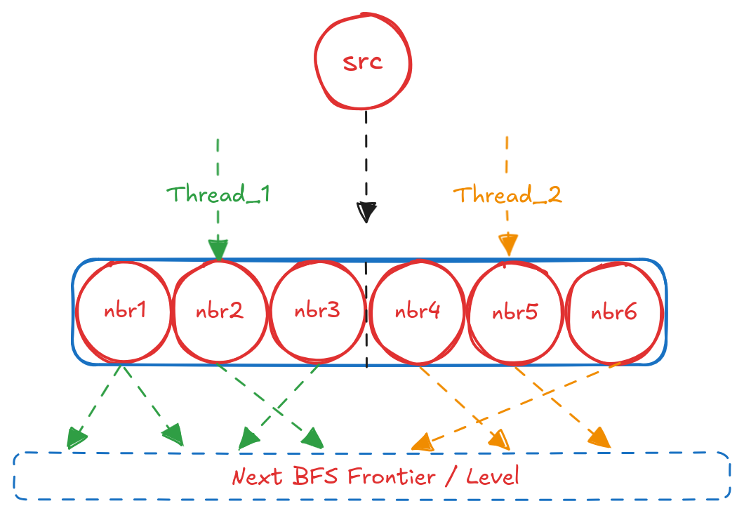
Since we are computing the unweighted shortest path, the appropriate algorithm is the classic breadth-first search (BFS). In the single-threaded setting, BFS is naturally implemented with a queue that tracks the current BFS level. In the parallel setting, however, the algorithm follows the bulk synchronous parallel (BSP) paradigm. The key idea is to have multiple threads explore the current frontier in parallel, while keeping track of which nodes have already been visited. Execution proceeds level by level: each thread is assigned a partition of the current frontier and expands all neighbors of the nodes within its partition. Once all threads complete their assigned work, they synchronize at a barrier, swap the current and next frontiers, and continue to the next BFS level.
Let’s outline the data structures required for our BFS algorithm:
(i) a global data structure, to track which nodes were visited already (global_visited)
(ii) a global data structure, to keep track of nodes in the current BFS level (curr_frontier)
(iii) a global data structure, to keep track of path lengths of destination nodes (path_length)
The most straightforward representation for (i)–(iii) is a set of arrays of size equal to the number of nodes in the graph. Updates must be visible across all threads, which we achieve using atomic operations. In addition, we require a data structure to hold the nodes discovered during the current level expansion, which will form the next frontier. For this, we use another array (next_frontier) and simply swap pointers between curr_frontier and next_frontier during the barrier phase. As threads traverse each level, their reads and writes to these shared structures must remain consistent. One naïve approach would be to protect each array (or buckets within them) with locks, but this would severely degrade parallel performance. Instead, we rely on atomic primitives— compare_and_exchange (also known as compare_and_swap, or CAS), along with atomic load and store—to provide lightweight, fine-grained synchronization.
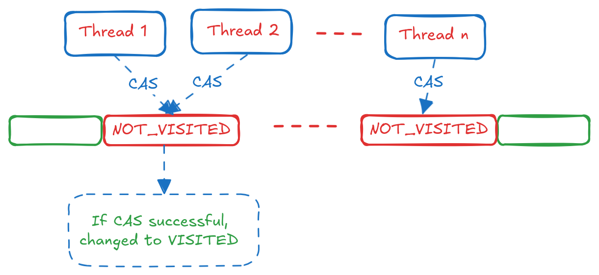
Consider the above scenario, where Thread 1 and Thread 2 encounter the same neighbour while expanding nodes from their respective partitions. Each thread will first check whether the neighbor has already been visited by reading its state from the global_visited array. If it is unvisited, both will attempt to mark it as visited. To make this safe, the read is performed using atomic_load. To guarantee that only one thread successfully updates the state, we use an atomic_cas (compare-and-swap) operation. The thread that “wins” the CAS proceeds to record the path length and mark the neighbor as part of the next frontier.
The pseudocode for this routine is shown below:
visited_nbrs(nbr_node) {
    state = atomic_read(global_visited[nbr_node])
    if (state == NOT_VISITED) {
        if (atomic_cas(&global_visited[nbr_node], state, VISITED) {
           atomic_store(&next_frontier[nbr_node], 1)
           atomic_store(&path_length[nbr_node], current_level + 1)
        }
    }
}
Each thread applies this subroutine to all neighbors until its frontier partition is exhausted. This simple lock-free design ensures correctness under concurrency and scales effectively with additional threads. In the next section, I’ll describe how we extend this approach to handle the more complex variable-length path queries.
Variable Length Path
The Cypher query we’re trying to parallelize here is:
MATCH p = (a:Person)-[r:Knows* 1..10]->(b:Person)
WHERE a.name = 'Alice'
RETURN p
To evaluate this query efficiently, we require the same parallel BFS traversal described in the previous section. Unlike the shortest-path query, however, the var-length path query introduces cycles: the same node can reappear at multiple BFS levels, and we must keep track of these repeated occurrences.
To see why this matters, let’s revisit our example graph:
Let’s enumerate what each BFS level would look like, starting from the source node (1):
Level 0: (1)
Level 1: (2), (3)
Level 2: (1), (4)
Level 3: (2), (3)
...
We notice that the same node can occur at multiple BFS levels. This means that associating each node with a single level or length is no longer sufficient. On top of that, this query doesn’t just return nodes—it returns paths. Let’s enumerate the paths of different lengths starting from node (1):
Length 1: (1)-[e1]->(2), (1)-[e2]->(3)
Length 2: (1)-[e1]->(2)-[e3]->(4), (1)-[e2]->(3)-[e4]->(4), (1)-[e1]->(2)-[e5]->(1)
Length 3: (1)-[e1]->(2)-[e5]->(1)-[e1]->(2), (1)-[e1]->(2)-[e5]->(1)-[e2]->(3)
...
When we start to enumerate the paths, a significant amount of redundancy becomes apparent. Nodes with multiple outgoing edges are duplicated across all paths they participate in, leading to repeated work and large intermediate results. The goal, therefore, is to avoid materializing these intermediate paths in full: each repeated node should be stored only once, with paths referencing it as needed. Consider representing all nodes in the graph as an array, and map the paths of Length 1 onto this structure:
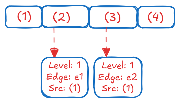
Each position in the array points to a block that contains information such as which BFS level it was encountered at, and the (edge ID, source node ID) that led to this node. When we visualize the paths one level deeper:
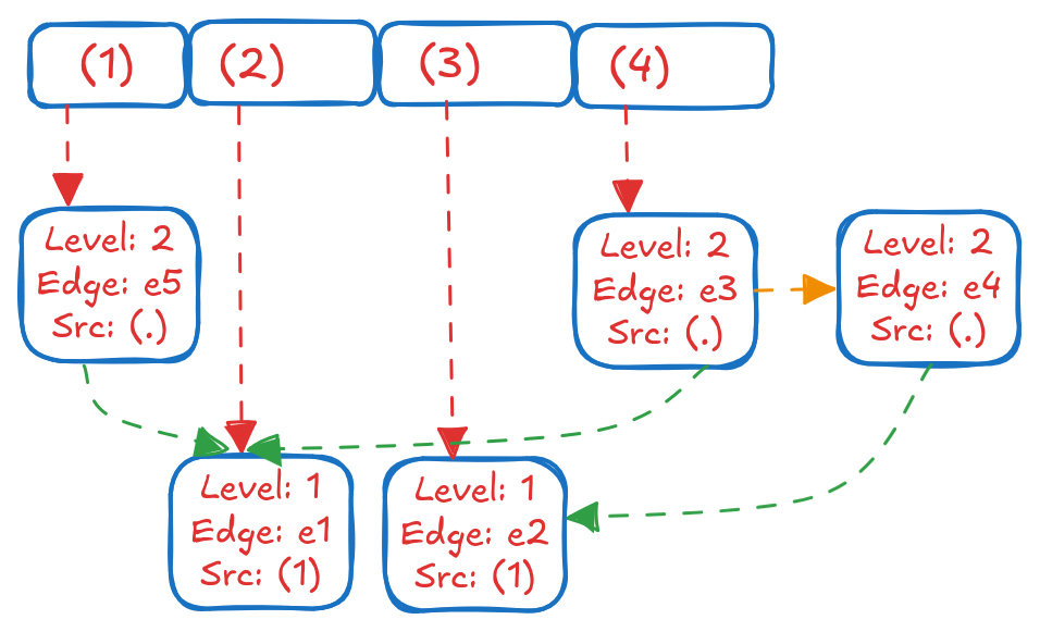
This representation avoids repeating Node (2) while keeping track of the 2 paths of Length 2 that start from it. This is useful in practice, especially when having to keep track of paths with cycles because it gives us a way to extract the paths when needed, but also avoids repeating nodes that are part of multiple paths at the same level. We can easily determine the paths by backtracking from the destination node to the source node using the (edge ID, source node ID) information stored in each block. We define 2 structs to store the information encapsulated in the blocks:
struct EdgeList {
    offset_t edge_offset
    EdgeListAndLevel* src
    EdgeList* next
}

struct EdgeListAndLevel {
    uint8_t bfs_level
    EdgeListAndLevel *next_level
    EdgeList* top
}
We are essentially moving towards a 2-D structure that grows vertically (BFS levels) and horizontally (all edges at a level). The EdgeListAndLevel struct is a linked list that goes deep and keeps track of specific levels a node was encountered. The EdgeList struct is a linked list that grows sideways and keeps track of all edges that led to that node, and their parent node from the previous level. The flow chart for the algorithm works is as follows:
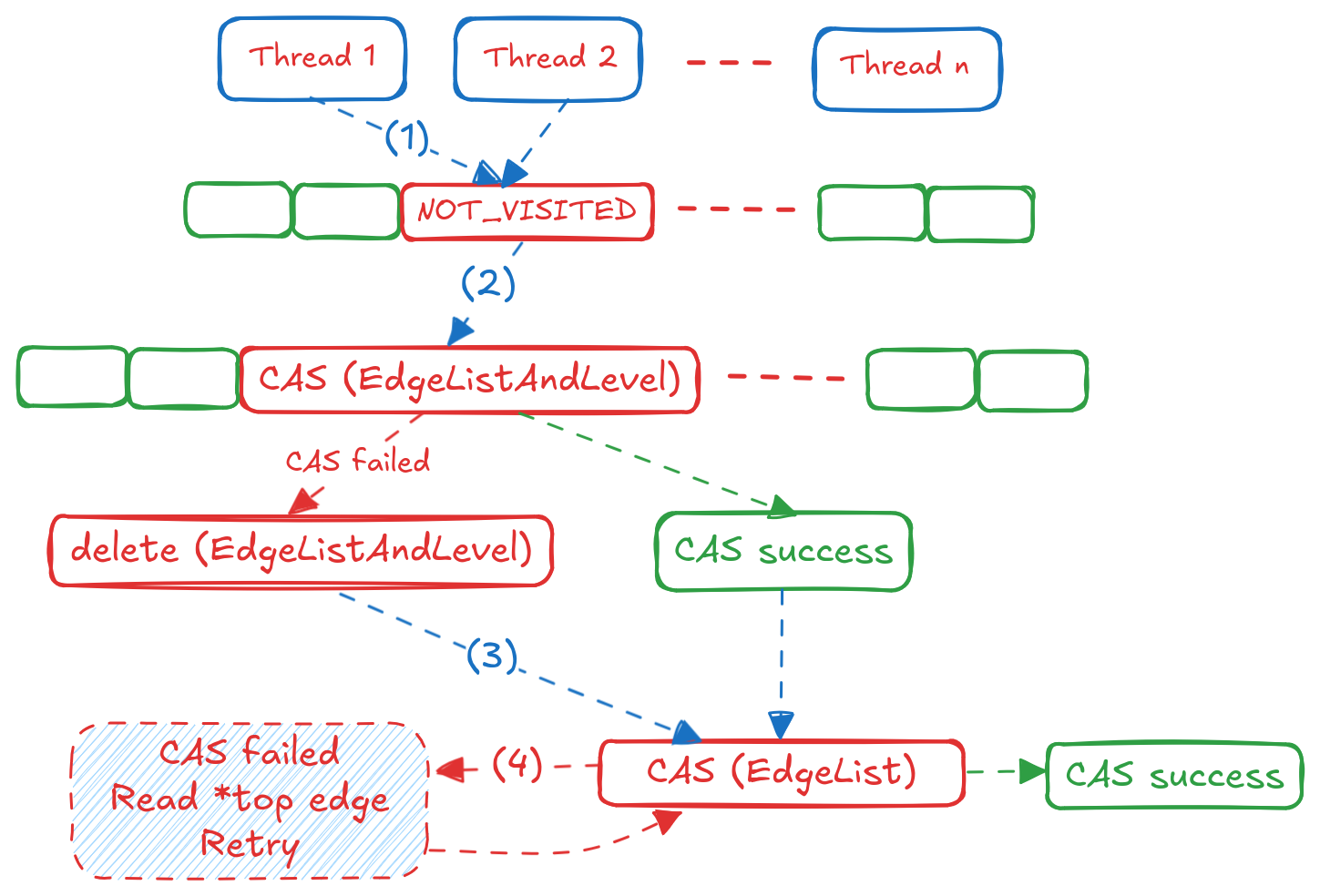
This is sufficiently complex, so let’s break it down step by step:
- Each Thread explores its partition of the current BFS level / frontier as before
- Unlike shortest path, in var-len queries nodes need not be marked visited only once, and can be visited multiple times at different levels. We still use the
global_visitedarray to mark if a node is visited at least once by any Thread and reset at the end of a BFS level (NOT_VISITEDchanged toVISITED). This is step(1)in the flow chart. - Now we need to check if the node was already encountered at the current BFS level. This is step
(2)in the flow chart. If it was not, we create a newEdgeListAndLevelstruct for this level and try to insert it into the linked list of levels for this node using anatomic_casoperation. If we succeed, we proceed to step(3). If we fail, it means another Thread already inserted a struct for this level concurrently. The Threads delete the struct they created and read the correctEdgeListAndLevelfrom the node position in the array. - In step
(3), we create a newEdgeListstruct for the edge that led to this node and try to insert it into the linked list of edges for this level using anatomic_casoperation. If we succeed, we are done processing this neighbour. If we fail, it means another Thread inserted an edge concurrently, so we read the updatedtophead pointer of theEdgeListAndLevelblock and try again until we succeed. This is step(4)in the flow chart. - Once all neighbours of all nodes in the current frontier are processed, we hit the barrier, swap the frontiers and move to the next BFS level.
Step (3) can be slightly optimized by reducing the number of memory allocations. Instead of allocating a new EdgeList struct for every neighbour, we can make a single large allocation for the entire partition of neighbours that a Thread is processing and make the EdgeList structs point to the appropriate offset in this large allocation. We call these large EdgeList allocations EdgeListSegments. For storing the EdgeListAndLevel structs per node, we use an array of pointers of size (total nodes) in the graph, and perform atomic operations to ensure all updates are visible to every thread. The pseudocode for processing each neighbour is as follows:
visited_nbrs(nbr_node, nbr_offset, edge_offset, src_node_level) {

    // Step (1) in flow chart
    state = atomic_read(global_visited[nbr_node])
    if (state == NOT_VISITED) {
        if (atomic_cas(&global_visited[nbr_node], state, VISITED)) {
            atomic_store(&next_frontier[nbr_node], 1)
        }
    }

    // Step (2) in flow chart
    node_level = NodeEdgeListAndLevels[nbr_node]
    if (node_level == NULL || node_level.bfs_level != current_level) {
        new_level = new EdgeListAndLevel(current_level, node_level, NULL)
        if (!atomic_cas(&NodeEdgeListAndLevels[nbr_node], node_level, new_level)) {
            delete new_level
            node_level = atomic_load(&NodeEdgeListAndLevels[nbr_node])
        } else {
            node_level = new_level
        }
    }

    // Step (3) in flow chart
    EdgeListSegment.edge_list_block[nbr_offset].edge_offset = edge_offset
    EdgeListSegment.edge_list_block[nbr_offset].src = src_node_level
    curr_top = atomic_load(&node_level.top)
    EdgeListSegment.edge_list_block[nbr_offset].next = curr_top

    // Step (4) in flow chart
    while (!atomic_cas(&node_level.top, curr_top, &EdgeListSegment.edge_list_block[nbr_offset])) {
        curr_top = atomic_load(&node_level.top)
        EdgeListSegment.edge_list_block[nbr_offset].next = curr_top
    }
}
This covers technical details of the lock-free variable length query algorithm for returning paths. Now lets look at some of the caveats of these techniques and what challenges we faced while implementing these algorithms in practice.
So, what’s the catch?
I just described two “fancy” algorithms that are fast, lock-free and scale well with more threads. But what’s the catch? Are there any drawbacks to these techniques ? There’s quite a few actually, and I’ll go through them one by one:
Memory Consumption: If it was not clear already, both algorithms use a lot of large arrays of size (total nodes) in the graph. This is not a problem for small graphs, but for large graphs with billions of nodes, this can be a problem. Some of the arrays can be optimized to be bitmaps such as the
global_visitedandnext_Frontierarray, but others such as theNodeEdgeListAndLevelsarray store a pointer per node which cannot be reduced. The problem with using bitmaps is that atomic operations on bits are not natively supported by hardware, so we have to useatomic_cason the entire byte / word, leading to more contention. The variable length query uses a lot more memory because of the linked list structures it maintains per node that grows vertically and horizontally.Memory Allocations: The var-length query algorithm needs to allocate a lot of small structures (
EdgeListAndLevel,EdgeList) during traversal. Even with the optimization of allocating large segments, to reduce theEdgeListallocations, the number of allocations remains high due to a new allocation needed per node for every level it is encountered (theEdgeListAndLevelstruct block).We initially benchmarked our var-length algorithm in Kùzu on the
LiveJournalgraph, on a machine with 16 physical cores (32 logical cores) for the following query:
    MATCH (a:lj_node)-[r:lj_rel* 1..5]->(b:lj_node)
    WHERE a.id < 50 AND b.id > 4847070
    RETURN r;
The query searches for paths upto a depth of 5, for 50 sources and 500 destinations and returns all paths. The result set contains 138,471 paths. We ran this query with the standard malloc allocator and compared it to jemalloc (a high performance memory allocator) for comparison:
| malloc | jemalloc | |
|---|---|---|
| Cold Run | 58 seconds | 27 seconds |
| Warm Run | 30 seconds | 26 seconds |
| malloc | jemalloc | |
|---|---|---|
| Peak | 75 GB | 47 GB |
| Post-Query | 70 GB | 11 GB |
With jemalloc the cold start runtime is 2x faster and peak memory usage is 1.6x lower. The post-query memory footprint is way lower with jemalloc because it returns memory to the OS more aggressively than standard malloc, which does not release memory back to the OS. The key takeaway here is that using a high performance memory allocator is crucial for this algorithm and lock-free algorithms in general to be performant in practice. You can write the most optimal lock-free algorithm, but if your memory allocator is not up to the task, you will not see the benefits in practice.
There’s a simple way to reduce the memory consumption of both algorithms, by reducing the concurrency level. When we limit the number of concurrent sources running in parallel to only 1 src node, the same query runs in 62 seconds and consumes only 5 GB peak memory (using jemalloc). The trade-off here is that the runtime is 2.3x slower. In a typical database setting, the best practice would be to allocate memory using a unified memory allocator that strictly keeps track of how much memory a query is using, and limit the concurrency level based on the memory budget.